Introducing the Power Grid Optimizer

This page gives an introduction to the Power Grid Optimizer (PGO), including the following topics:

The motivation for developing and using the PGO
Grid Configuration as an Optimal Power Flow problem
The PGO, what it is, and how it can be used

This is meant as an introductionary text. For a full overview of PGO documentation, please see the main PGO documentation page.

Motivation

DSOs aim to develop and manage their distribution grid in a way that is cost efficient, maximizes customer satisfaction, and minimizes disruptions due to faults or maintenance.

The power grid contains a number of different resources, such as switches, transformers, batteries, controllable consumption or production (other flexibility sources) that each can be configured or exploited in different ways. Here, we use the term “grid configuration” to mean the total configuration of all these resources in the power grid.

The choice of grid configuration greatly impacts the grid’s reliability and cost-efficiency. Making the right decisions, both in grid planning and daily operations, therefore require the ability to determine a grid configuration that is optimal in some sense, e.g. with respect to power loss, reliability (incl. reserve capacity and expected loss of energy not delivered (in Norway: “KILE”)), load distribution, cost of flexibility, customer satisfaction, and other quality measures. Moreover, such an “optimal” configuration must be found within the time constraints of the planning situation.

The ability to efficiently determine the best possible configuration, both in long term planning and in short term grid management, is therefore critical to successful DSO operations.

Grid Configuration is an Optimal Power Flow problem

Determining a robust and cost-efficient configuration is, however, a hard optimization problem to solve. This is due to a combination of factors:

Since there are so many configurable resources (e.g. switches), and two (or more) settings for each, the problem has very many discrete (often binary) configuration variables. This, in turn, gives the problem a high combinatorial complexity; i.e. there are very many possible configurations to choose from.
The uncertainty inherent in the forecasted demand, renewable production, etc.
The need to ensure that physical grid constraints are satisfied, such as voltage and current limits on different components. This means that to evaluate each individual configuration (solution), the power flow equations must be solved, which is time consuming.

To enable decision support tools that can solve such “optimal power flow” problems, for realistic grid sizes and planning situations, there is a great need for further research into optimization methods, both exact and heuristic. This falls under overlapping research fields such as Operations Research and Artificial Intelligence.

For a introduction to Optimal Powerflow Problems, see, for example Frank and Rebennack’s paper “An introduction to optimal power flow: Theory, formulation, and examples” [1].

The Power Grid Optimiser software

As explained in the introduction, the PGO is a software for computing an optimal (or near optimal) grid configuration. In the PGO, this task is formulated as a combinatorial optimisation problem, and solved using a suite of suitable search methods, both exact and approximate. By solving variations of this problem efficiently, the technology enables considerable savings on several levels in DSO/TSO operations, ranging from long term investment analysis, through a dynamic adaptation of the grid based on short term prognosis, to here-and-now re-configuration during maintenance or fault corrections. We expect that usage of the PGO may achieve significant savings and added grid robustness, as compared to the present practice of evaluating only a few manually created candidate configurations.

This text contains a brief introduction to what the PGO is, what it can do, and how to use it. We assume that you are already familiar with the background section.

The current version

Currently, the PGO supports two main applications:

The computation of a static “default configuration” for a distribution grid. Today, such default configurations are normally chosen based on a manual investigation of a very small number of possible configurations. It is likely that configuration chosen in this way is not an optimal one, and that a better configuration may be found with the proper tools.
The computation of a configuration schedule. That is, a sequence of configurations over a number of time steps. This can be used in daily operations to dynamically make minor adjustments to the near-future configurations. The aim is to remove predicted bottlenecks that appear due to variation in demand, local production, grid capacity, and/or component vulnerability (due to weather), and so ensure a stable delivery. Furthermore, the PGO may be used to evaluate any existing configuration, by computing the associated power flow and measuring the relevant quality criteria.

Note that while our scope is “grid configuration” in the widest sence, including all configurable grid resources, the first (current) version of the PGO, considers only switch settings. Extending the set of decision variables to other grid resources, and for other specific planning tasks, are subjects for continued research.

Using the PGO service

You can access the PGO either as code, or by downloading a docker image; see the github PGO Readme.

For a fast touch-and-feel introduction, please try out our web application. This is a simple web-based client which you can use to access the PGO server and try out some grid configuration optimisation. The user manual for the web application is here.

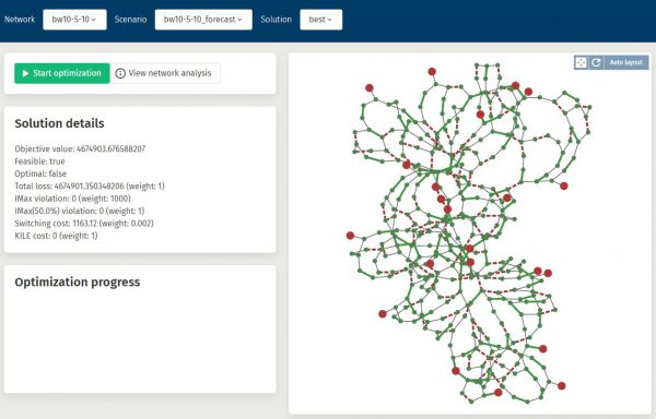
The API

The PGO can be used in two ways, depending on user preferences:

In process, through a .NET based API
As a service, through an http based API (see Figure 2).

Simply put, either of these API can be used programmatically to:

Upload a grid definition to the PGO, e.g. taking data from third party software.
Create an optimization session, by uploading a forecasted or estimated demand for each consumer
Define the optimisation criterion by setting relative weight for quality measures such as “thermal loss” or “Expected cost of energy not delivered”.
Run an optimisation for this session, to produce a (near) optimal configuration for the associated demand.
Retrieve the resulting configuration, along with the associated power flow, e.g. for visualization or further analysis.
Upload any configuration that may have been otherwise produced outside the PGO, and have it evaluated in terms of power flow and configuration quality.


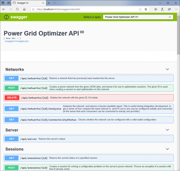The service comes with a complete on-line API reference documentation

For more detailed information about how to integrate and use the PGO service in a production setting, take a look at the main PGO documentation page. More technical detail, and direct access to the software, can be found at github.

Input data

The data that are necessary for using the PGO are:

The distribution network data, including grid topology and the necessary physical properties of switches, lines, buses, and transformers. These are typically taken from the DSO’s NIS or SCADA systems.
Power demand predictions: When choosing a static default configuration, this will be a single number for each of the consumers. Depending on what you want to compute; these can represent a normal average situation, a winter scenario, a worst-case scenario, etc. For more dynamic and short term planning, a time series can be provided for each consumer, giving a predicted demand on (for example) an hourly basis.

The PGO supports two data formats, for separate purposes:

A proprietary json-based format for defining the grid data. This is the easiest to use, e.g. in researching new optimization or power flow computation methods.
A CIM-based format, with JSON-LD. CIM (Common Information Model) is an industry standard for representing power networks and associated data. This may be the best format to use when integrating with other CIM-compatible applications.

More information about the data formats can be found on github.

Model and algorithms

This section gives a high-level overview of how we have defined the grid configuration optimisation problem, and the various research challenges that we have addressed to solve it.

As mentioned above, we limit our definition of “grid configuration” to determining an optimal setting for each switch in the grid. In Norway, it is normally assumed that feasible configurations must be “radial”, in the sense that in the resulting (configured) grid there is exactly one path from each bus to a substation (i.e., each bus gets power through exactly one connecting path from the higher-voltage transmission grid). Furthermore, a feasible configuration must comply with current and voltage limits set for the various grid components. Therefore, to determine whether a configuration is feasible, the corresponding power flow must be computed for the entire grid. This computation is also the basis for evaluating the quality of the configuration, e.g. in terms of robustness or power loss.

The number of possible configurations is 2ⁿ, where n is the number of available switches. This “exponentially exploding” number of possible configurations makes this a “hard” combinatorial optimization problem. Solving the problem is made even more challenging by the need to compute the power flow for every configuration that is considered, a computation that in itself is time consuming.

To develop this prototype, our challenge was to:

Develop an efficient (heuristic) optimisation algorithm for grid configuration
Develop an efficient power flow computation method, for use in the optimisation algorithm
Develop an easy-to-use API, to facilitate integration with DSO legacy systems.
Testing of the PGO prototype on real distribution net data.

The PGO employs a “meta-heuristic” search method for solving the optimisation algorithm, based on a fast heuristic for constructing radial solutions, a local search for improving such solutions, and a “ruin-and-recreate” diversification strategy. For the power flow calculations, we use an efficient “iterative” implementation of the “backward/forward sweep” algorithm [2,3], the efficiency of which rests on the assumption of radiality. Other power flow algorithms are also included that can handle also “non-radial” configurations, but these are not competitive for radial networks.

References

[1] Frank, Stephen, and Steffen Rebennack. “An introduction to optimal power flow: Theory, formulation, and examples.” IIE transactions 48.12 (2016): 1172-1197.

[2] Luo, Guang-Xiang, and Adam Semlyen. “Efficient load flow for large weakly meshed networks.” IEEE Transactions on Power Systems 5.4 (2002): 1309-1316.

[3] Shirmohammadi, Dariush, et al. “A compensation-based power flow method for weakly meshed distribution and transmission networks.” IEEE Transactions on power systems 3.2 (2002): 753-762.